Zernike polynomials

In mathematics, the Zernike polynomials are a sequence of polynomials that are orthogonal on the unit disk. Named after Frits Zernike, they play an important role in beam optics.

1 Definitions
- 1.1 Other Representations
2 Formulas
- 2.1 Orthogonality
- 2.2 Symmetries
3 Examples
4 Applications
5 Higher Dimensions
6 See also
7 Notes
8 References
9 External links

Definitions

There are even and odd Zernike polynomials. The even ones are defined as

$Z^{m}_n(\rho,\varphi) = R^m_n(\rho)\,\cos(m\,\varphi) \!$

and the odd ones as

$Z^{-m}_n(\rho,\varphi) = R^m_n(\rho)\,\sin(m\,\varphi), \!$

where m and n are nonnegative integers with n≥m, φ is the azimuthal angle, and ρ is the radial distance $0\le\rho\le 1$ . The radial polynomials R^m_n are defined as

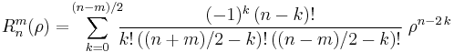
$R^m_n(\rho) = \! \sum_{k=0}^{(n-m)/2} \!\!\! \frac{(-1)^k\,(n-k)!}{k!\,((n%2Bm)/2-k)!\,((n-m)/2-k)!} \;\rho^{n-2\,k}$

for n − m even, and are identically 0 for n − m odd.

Other Representations

Rewriting the ratios of factorials in the radial part as products of binomials shows that the coefficients are integer numbers:

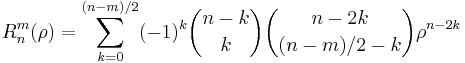$R_n^m(\rho)=\sum_{k=0}^{(n-m)/2}(-1)^k \binom{n-k}{k} \binom{n-2k}{(n-m)/2-k} \rho^{n-2k}$ .

A notation as terminating Gaussian Hypergeometric Functions is useful to reveal recurrences, to demonstrate that they are special cases of Jacobi polynomials, to write down the differential equations, etc.:

$R_n^m(\rho)= \binom{n}{(n%2Bm)/2} \rho^n {}_2F_{1}\left(-\frac{n%2Bm}{2},-\frac{n-m}{2};-n;\rho^{-2}\right)$

$= (-1)^{(n%2Bm)/2}\binom{(n%2Bm)/2}{(n-m)/2}\rho^m {}_2F_{1}\left(1%2Bn,1-\frac{n-m}{2};1%2B\frac{n%2Bm}{2};\rho^2\right)$

for n − m even.

Applications often involve linear algebra, where integrals over products of Zernike polynomials and some other factor build the matrix elements. To enumerate the rows and columns of these matrices by a single index, a conventional mapping of the two indices n and m to a single index j has been introduced by Noll. The table of this association $Z_n^m \rightarrow Z_j$ starts as follows (sequence A176988 in OEIS)

n,m	0,0	1,1	1,-1	2,0	2,-2	2,2	3,-1	3,1	3,-3	3,3
j	1	2	3	4	5	6	7	8	9	10
n,m	4,0	4,2	4,-2	4,4	4,-4	5,1	5,-1	5,3	5,-3	5,5
j	11	12	13	14	15	16	17	18	19	20

The rule is that the even Z (with azimuthal part $\cos(m\varphi)$ ) obtain even indices j, the odd Z odd indices j. Within a given n, lower values of m obtain lower j.

Formulas

Orthogonality

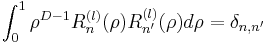
The orthogonality in the radial part reads

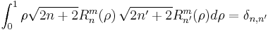$\int_0^1 \rho \sqrt{2n%2B2}R_n^m(\rho)\,\sqrt{2n'%2B2}R_{n'}^{m}(\rho)d\rho = \delta_{n,n'}$ .

Orthogonality in the angular part is represented by

$\int_0^{2\pi} \cos(m\varphi)\cos(m'\varphi)d\varphi=\epsilon_m\pi\delta_{|m|,|m'|}$ ,

$\int_0^{2\pi} \sin(m\varphi)\sin(m'\varphi)d\varphi=(-1)^{m%2Bm'}\pi\delta_{|m|,|m'|};\quad m\neq 0$ ,

$\int_0^{2\pi} \cos(m\varphi)\sin(m'\varphi)d\varphi=0$ ,

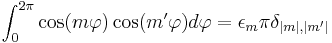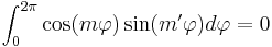where $\epsilon_m$ (sometimes called the Neumann factor because it frequently appears in conjunction with Bessel functions) is defined as 2 if $m=0$ and 1 if $m\neq 0$ . The product of the angular and radial parts establishes the orthogonality of the Zernike functions with respect to both indices if integrated over the unit disk,

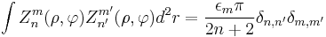$\int Z_n^m(\rho,\varphi)Z_{n'}^{m'}(\rho,\varphi)d^2r =\frac{\epsilon_m\pi}{2n%2B2}\delta_{n,n'}\delta_{m,m'}$ ,

where 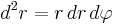$d^2r=r\,dr\,d\varphi$ is the Jacobian of the circular coordinate system, and where $n-m$ and $n'-m'$ are both even.

A special value is

$R_n^m(1)=1$ .

Symmetries

The parity with respect to reflection along the x axis is

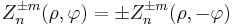
$Z_n^{\pm m}(\rho,\varphi)=\pm Z_n^{\pm m}(\rho,-\varphi)$ .

The parity with respect to point reflection at the center of coordinates is

$Z_n^m(\rho,\varphi) = (-1)^m Z_n^m(\rho,\varphi%2B\pi)$ ,

where $(-1)^m$ could as well be written $(-1)^n$ because $n-m$ is even for the relevant, non-vanishing values. The radial polynomials are also either even or odd:

$R_n^m(\rho)=(-1)^m R_n^m(-\rho)$ .

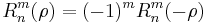The periodicity of the trigonometric functions implies invariance if rotated by multiples of $2\pi/m$ radian around the center:

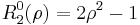
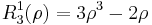
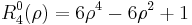
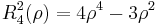
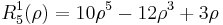
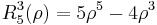
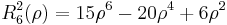
$Z_n^m(\rho,\varphi%2B2\pi k/m)=Z_n^m(\rho,\varphi),\quad k= 0, \pm 1,\pm 2,\ldots$ .

Examples

The first few Radial polynomials are:

$R^0_0(\rho) = 1 \,$

$R^1_1(\rho) = \rho \,$

$R^0_2(\rho) = 2\rho^2 - 1 \,$

$R^2_2(\rho) = \rho^2 \,$

$R^1_3(\rho) = 3\rho^3 - 2\rho \,$

$R^3_3(\rho) = \rho^3 \,$

$R^0_4(\rho) = 6\rho^4 - 6\rho^2 %2B 1 \,$

$R^2_4(\rho) = 4\rho^4 - 3\rho^2 \,$

$R^4_4(\rho) = \rho^4 \,$

$R^1_5(\rho) = 10\rho^5 - 12\rho^3 %2B 3\rho \,$

$R^3_5(\rho) = 5\rho^5 - 4\rho^3 \,$

$R^5_5(\rho) = \rho^5 \,$

$R^0_6(\rho) = 20\rho^6 - 30\rho^4 %2B 12\rho^2 - 1 \,$

$R^2_6(\rho) = 15\rho^6 - 20\rho^4 %2B 6\rho^2 \,$

$R^4_6(\rho) = 6\rho^6 - 5\rho^4 \,$

$R^6_6(\rho) = \rho^6. \,$

Applications

The functions are a basis defined over the circular support area, typically the pupil planes in classical optical imaging at optical and infrared wavelengths through systems of lenses and mirrors of finite diameter. Their advantage are the simple analytical properties inherited from the simplicity of the radial functions and the factorization in radial and azimuthal functions; this leads for example to closed form expressions of the two-dimensional Fourier transform in terms of Bessel Functions. Their disadvantage, in particular if high n are involved, is the unequal distribution of nodal lines over the unit disk, which introduces ringing effects near the perimeter $\rho\approx 1$ , which often leads attempts to define other orthogonal functions over the circular disk.

In precision optical manufacturing, Zernike polynomials are used to characterize higher-order errors observed in interferometric analyses, in order to achieve desired system performance.

In optometry and ophthalmology the Zernike polynomials are used to describe aberrations of the cornea or lens from an ideal spherical shape, which result in refraction errors.

They are commonly used in adaptive optics where they can be used to effectively cancel out atmospheric distortion. Obvious applications for this are IR or visual astronomy, and Satellite imagery. For example, one of the zernike terms (for m = 0, n = 2) is called 'de-focus'. By coupling the output from this term to a control system, an automatic focus can be implemented.

Another application of the Zernike polynomials is found in the Extended Nijboer-Zernike (ENZ) theory of diffraction and aberrations.

Zernike polynomials are widely used as basis functions of image moments.

Higher Dimensions

The concept translates to higher dimensions $D$ if multinomials $x_1^ix_2^j\cdots x_D^k$ in Cartesian coordinates are converted to hyperspherical coordinates, $\rho^s$ , $s\le D$ , multiplied by a product of Jacobi Polynomials of the angular variables. In $D=3$ dimensions, the angular variables are Spherical harmonics, for example. Linear combinations of the powers $\rho^s$ define an orthogonal basis $R_n^{(l)}(\rho)$ satisfying

$\int_0^1 \rho^{D-1}R_n^{(l)}(\rho)R_{n'}^{(l)}(\rho)d\rho = \delta_{n,n'}$ .

(Note that a factor $\sqrt{2n%2BD}$ is absorbed in the definition of $R$ here, whereas in $D=2$ the normalization is chosen slightly differently. This is largely a matter of taste, depending on whether one wishes to maintain an integer set of coefficients or prefers tighter formulas if the orthogonalization is involved.) The explicit representation is

References

- Born and Wolf, "Principles of Optics", Oxford: Pergamon, 1970
- Weisstein, Eric W., "Zernike Polynomial" from MathWorld.
- Campbell, C. E. (2003). "Matrix method to find a new set of Zernike coefficients form an original set when the aperture radius is changed". J. Opt. Soc. Am. A 20 (2): 209. Bibcode 2003JOSAA..20..209C. doi:10.1364/JOSAA.20.000209.
- Cerjan, C. (2007). "The Zernike-Bessel representation and its application to Hankel transforms". J. Opt. Soc. Am. A 24 (6): 1609. Bibcode 2007JOSAA..24.1609C. doi:10.1364/JOSAA.24.001609.
- Comastri, S. A.; Perez, L. I.; Perez, G. D.; Martin, G.; Bastida Cerjan, K. (2007). "Zernike expansion coefficients: rescaling and decentering for different pupils and evaluation of corneal aberrations". J. Opt. A: Pure Appl. Opt. 9 (3): 209. Bibcode 2007JOptA...9..209C. doi:10.1088/1464-4258/9/3/001.
- Conforti, G. (1983). "Zernike aberration coefficients from Seidel and higher-order power-series coefficients". Opt. Lett. 8 (7): 407–408. Bibcode 1983OptL....8..407C. doi:10.1364/OL.8.000407. http://www.opticsinfobase.org/abstract.cfm?URI=ol-8-7-407.
- Dai, G-m.; Mahajan, V. N. (2007). "Zernike annular polynomials and atmospheric turbulence". J. Opt. Soc. Am. A 24: 139. Bibcode 2007JOSAA..24..139D. doi:10.1364/JOSAA.24.000139. http://www.opticsinfobase.org/abstract.cfm?URI=josaa-24-1-139.
- Dai, G-m. (2006). "Scaling Zernike expansion coefficients to smaller pupil sizes: a simpler formula". J. Opt. Soc. Am. A 23 (3): 539. Bibcode 2006JOSAA..23..539D. doi:10.1364/JOSAA.23.000539. http://www.opticsinfobase.org/abstract.cfm?URI=josaa-23-3-539.
- Díaz, J. A.; Fernández-Dorado, J.; Pizarro, C.; Arasa, J. (2009). "Zernike Coefficients for Concentric, Circular, Scaled Pupils: An Equivalent Expression". Journal of Modern Optics 56 (1): 149–155. Bibcode 2009JMOp...56..149D. doi:10.1080/09500340802531224.
- Díaz, J. A.; Fernández-Dorado, J.. "Zernike Coefficients for Concentric, Circular, Scaled Pupils". http://demonstrations.wolfram.com/ZernikeCoefficientsForConcentricCircularScaledPupils/. from The Wolfram Demonstrations Project.
- Herrmann, J. (1981). "Cross coupling and aliasing in modal wave-front estimation". J. Opt. Soc. Am. 71 (8): 989. Bibcode 1981JOSA...71..989H. doi:10.1364/JOSA.71.000989. http://www.opticsinfobase.org/abstract.cfm?URI=josa-71-8-989.
- Hu, P. H.; Stone, J.; Stanley, T. (1989). "Application of Zernike polynomials to atmospheric propagation problems". J. Opt. Soc. Am. A 6 (10): 1595. Bibcode 1989JOSAA...6.1595H. doi:10.1364/JOSAA.6.001595. http://www.opticsinfobase.org/abstract.cfm?URI=josaa-6-10-1595.
- Kintner, E. C. (1976). "On the mathematical properties of the Zernike Polynomials". Opt. Acta 23 (8): 679. Bibcode 1976AcOpt..23..679K. doi:10.1080/713819334.
- Lawrence, G. N.; Chow, W. W. (1984). "Wave-front tomography by Zernike Polynomial decomposition". Opt. Lett. 9 (7): 267. Bibcode 1984OptL....9..267L. doi:10.1364/OL.9.000267. http://www.opticsinfobase.org/abstract.cfm?URI=ol-9-7-267.
- Lundström, L.; Unsbo, P. (2007). "Transformation of Zernike coefficients: scaled, translated and rotated wavefronts with circular and elliptical pupils". J. Opt. Soc. Am. A 24 (3): 569. Bibcode 2007JOSAA..24..569L. doi:10.1364/JOSAA.24.000569.
- Mahajan, V. N. (1981). "Zernike annular polynomials for imaging systems with annular pupils". J. Opt. Soc. Am. 71: 75. Bibcode 1981JOSA...71...75M. doi:10.1364/JOSA.71.000075. http://www.opticsinfobase.org/abstract.cfm?URI=josa-71-1-75.
- Mathar, R. J. (2007). "Third Order Newton's Method for Zernike Polynomial Zeros". arXiv:0705.1329 [math.NA]. Bibcode 2007arXiv0705.1329M.
- Mathar, R. J. (2009). "Zernike Basis to Cartesian Transformations". Serb. Astron. J. 179 (179): 107–120. Bibcode 2009SerAj.179..107M. doi:10.2298/SAJ0979107M.
- Noll, R. J. (1976). "Zernike polynomials and atmospheric turbulence". J. Opt. Soc. Am. 66 (3): 207. Bibcode 1976JOSA...66..207N. doi:10.1364/JOSA.66.000207.
- Prata Jr, A.; Rusch, W. V. T. (1989). "Algorithm for computation of Zernike polynomials expansion coefficients". Appl. Opt. 28 (4): 749. Bibcode 1989ApOpt..28..749P. doi:10.1364/AO.28.000749. http://www.opticsinfobase.org/abstract.cfm?URI=ao-28-4-749.
- Schwiegerling, J. (2002). "Scaling Zernike expansion coefficients to different pupil sizes". J. Opt. Soc. Am. A 19 (10): 1937. Bibcode 2002JOSAA..19.1937S. doi:10.1364/JOSAA.19.001937. http://www.opticsinfobase.org/abstract.cfm?URI=josaa-19-10-1937.
- Sheppard, C. J. R.; Campbell, S.; Hirschhorn, M. D. (2004). "Zernike expansion of separable functions in Cartesian coordinates". Appl. Opt. 43 (20): 3963. Bibcode 2004ApOpt..43.3963S. doi:10.1364/AO.43.003963. http://www.opticsinfobase.org/abstract.cfm?URI=ao-43-20-3963.
- Shu, H.; Luo, L.; Han, G.; Coatrieux, J.-L. (2006). "General method to derive the relationship between two sets of Zernike coefficients corresponding to different aperture sizes". J. Opt. Soc. Am. A 23 (8): 1960. Bibcode 2006JOSAA..23.1960S. doi:10.1364/JOSAA.23.001960. http://www.opticsinfobase.org/abstract.cfm?URI=josaa-23-8-1960.
- Swantner, W.; Chow, W. W. (1994). "Gram-Schmidt orthogonalization of Zernike polynomials for general aperture shapes". Appl. Opt. 33 (10): 1832. Bibcode 1994ApOpt..33.1832S. doi:10.1364/AO.33.001832. http://www.opticsinfobase.org/abstract.cfm?URI=ao-33-10-1832.
- Tango, W. J. (1977). "The circle polynomials of Zernike and their application in optics". Appl. Phys. A 13 (4): 327. Bibcode 1977ApPhy..13..327T. doi:10.1007/BF00882606.
- Tyson, R. K. (1982). "Conversion of Zernike aberration coefficients to Seidel and higher-order power series aberration coefficients". Opt. Lett. 7 (6): 262. Bibcode 1982OptL....7..262T. doi:10.1364/OL.7.000262. http://www.opticsinfobase.org/abstract.cfm?URI=ol-7-6-262.
- Wang, J. Y.; Silva, D. E. (1980). "Wave-front interpretation with Zernike Polynomials". Appl. Opt. 19 (9): 1510. Bibcode 1980ApOpt..19.1510W. doi:10.1364/AO.19.001510. http://www.opticsinfobase.org/abstract.cfm?URI=ao-19-9-1510.
- Barakat, R. (1980). "Optimum balanced wave-front aberrations for radially symmetric amplitude distributions: Generalizations of Zernike polynomials". J. Opt. Soc. Am. 70 (6): 739. Bibcode 1980JOSA...70..739B. doi:10.1364/JOSA.70.000739. http://www.opticsinfobase.org/abstract.cfm?URI=josa-70-6-739.
- Bhatia, A. B.; Wolf, E. (1952). "The Zernike circle polynomials occurring in diffraction theory". Proc. Phys. Soc. B 65 (11): 909. Bibcode 1952PPSB...65..909B. doi:10.1088/0370-1301/65/11/112.
- ten Brummelaar, T. A. (1996). "Modeling atmospheric wave aberrations and astronomical instrumentation using the polynomials of Zernike". Opt. Commun. 132 (3–4): 329. Bibcode 1996OptCo.132..329T. doi:10.1016/0030-4018(96)00407-5.
- Novotni, M.; Klein, R. (2003). "3D Zernike Descriptors for Content Based Shape Retrieval". Proceedings of the 8th ACM Symposium on Solid Modeling and Applications: 216–225. doi:10.1145/781606.781639. http://www.cg.cs.uni-bonn.de/docs/publications/2003/novotni-2003-3d.pdf.
- Novotni, M.; Klein, R. (2004). "Shape retrieval using 3D Zernike descriptors". Computer Aided Design 36 (11): 1047–1062. doi:10.1016/j.cad.2004.01.005. http://www.cg.cs.uni-bonn.de/docs/publications/2004/novotni-2004-shape.pdf.